
Straight-Line Transect Survey Procedures
Straight-Line Transects
This approach is the most effective for creating accurate PO maps, however it requires a methodology that may be more time-consuming than the second approach. We recommend using two people for the survey - one to operate the gps unit, stay on the transect and enter data, and the other to scan for plants within 5 meters on either side of the transect. The process begins with the delineation of transects within the area's roads and extend (preferably for 2 km) at a right angle to those roads (see figure 5), a process which is completed in the office. Two kilometer transects were used in the Yellowstone Northern range, as it was difficult to consistently find areas that were greater than 2 km from any road. This length is preferred, however the distance should be consistent with the density of roads in the management area, and should be the same across all transects. The transects should start at random locations along each road in the management area. Once transect lines are defined, they are loaded into a GPS unit for easy following. We recommend using Trimble GeoXT GPS units with TerraSync as the data collection software. Next, one may either use a form with the following defined fields, or load our suggested data dictionary into each GPS unit. The fields for a plant point are as follows:
Note: When starting and ending a transect, record a plant point WITHOUT any attributes, which will delineate the beginning/end of the transect
a. Species 1 Name. This represents the target species of concern. In an automated data dictionary, it
would be presented as a drop-down menu. The fields presented are replicated for up
to 4 species
b. Patch Position 1. The position of the GPS unit in relation to the patch. A patch is defined as a collection
of plants that does not have any plants of the same species within 10 meters of its
boundary. Options are start, middle and end. A start is used when the end of a patch
cannot be visually identified from the beginning point. In such a case, one fills
out the species name and the patch position, and leaves the rest of the fields blank
(to be filled in at the end point). An end is used when one finally finds the end
of the long patch and does not find any other plants within 10 meters of that point.
When an end is used, it is also necessary to fill out all the other fields relating
to the patch. A middle is used when one can visually determine the boundaries of the
patch. In such a case, the user walks to the middle of the patch (along the transect)
to record a center point, and then enters the patch dimensions and other attributes
provided by the second team member.
c. Optional for monitoring purposes. Spatial Position 1. The options here are ind/scattered plants, discrete patches and
interconnected patch. Ind/scattered means that the plants are individually scattered
throughout the patch area, and do not appear to have any distinguishing clumps or
patterns. This designation is also used for individual plants of the target species.
One example of a plant that tends to usually fall under this category would be common
mullein. Discrete patches is used for patches that form in clumps or well-defined
polygons. Common Tansy is a species that often exhibits this characteristic. Interconnected
patch is used for species that are sometimes discrete, sometimes individual, but ultimately
tend to have a haphazard pattern of interconnected distribution. For example, cheatgrass
often forms in clumps, but also is strung along between these discrete patches as
individuals - thus it would be called interconnected.
d. Optional for monitoring purposes. Canopy Cover 1. This attribute represents mean percent cover for the patch. It is
a rough visual estimate.
e. Patch Length 1. The length of the patch in meters. Only recorded when creating a middle point.
f. Patch Width 1. The width of the patch in meters, averaged over the entire length of the patch.
g. Optional for monitoring purposes. Weed Density 1. Less than 1, 1 - 11, 12 - 32, 33 - 100, 101 - 316, 317 - 1000 per
square meter. The average number of individuals of the target species that occur in
a square meter in the patch. For example, if there was a 10 square meter patch, and
two square meters of that patch were occupied by 20 individuals each, then over the
whole patch the average density would be 40/10, or 4 individuals per square meter.
This would fall into the 1-11 category. To use the <1 category, a patch must have
a larger number of square meters than there are individuals. For example, if a patch
was 5 meters by 5 meters (25 square meters), but only had two individuals in each
corner, the number of individuals per average square meter would clearly be less than
one.
h. Latitude
i. Longitude
The above options are then repeated for species 2 - 4. If there are more than 4 species
at any one point (which can happen along roadsides) it is necessary to create another
plant point and then fill in the species 1-4 options again.
j. Species 2 Name
k. Patch Position 2
l. Etc...
How To Collect Data in the Field
Transects should be walked and survey observations made within a 10 m wide swath. When a target NIS is located, the dimensions (length and width) of the patch should be estimated. If the length is longer than can be visually determined, then the beginning of the patch is recorded as a "start" point and only the species needs to be entered in the list of fields. Otherwise, the user walks to the middle of the patch (staying on the transect line), and records the patch as a "middle" point, along with the spatial position, canopy cover, etc. If the patch for which the "start " point was created comes to an end, then an "end" point is created and all the data fields are filled out with estimates of the average values for the entire patch. For example, if a patch of cheatgrass (Bromus tectorum) is encountered, but only occurs in dense clumps within a 30 meter length (10 meter width) patch, then the number of stems per square meter needs to be estimated over the entire 300 square meter area to arrive at the density value. If there were 10 patches, each 1 square meter, with 100 stems in each, then the average density would be (100 stems per plot x 10 plots) / 300 m2 = 3.33 stems per m2 , or the 1 - 11 density category.
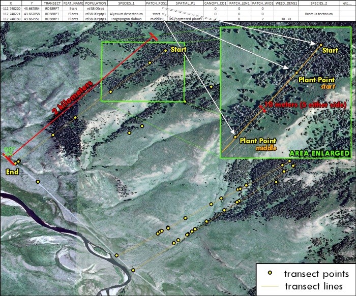
Figure 4. Diagram showing transect layouts and a representative attribute table.